RAG on vllm-gke

Note: This article is a continuation of Multi-Tier LLM Routing on GKE. The full codebase is available on GitHub: iheb24/vllm-gke.

Plain simple RAG. We wanted to deep dive RAG practices for a chat assistant, understand the components involved, how they communicate with each other, and which strategies make a RAG pipeline actually good. This article is based on research and input from Mohamed-Amine Bousahih, where we tested, observed, and exchanged ideas together.

The goal: add a RAG capability to my vllm-gke stack, able to index text documents in multiple formats. Two constraints carried over from the previous articles. GPU scale-to-zero must stay operative, and the retrieved knowledge must be usable by both the CPU (SLM) and the GPU tiers.

One note on intent. The theme of the corpus does not matter much to me, and theming was a hot subject in past years. The value shifted to the quality of what you retrieve. So I went quality-first: a small seed corpus, measured retrieval, and only then permission to scale content up.

First, unlearn three things

RAG stands for Retrieval-Augmented Generation. We thought it was really about the content: pick a vector database, index documents, done. We also intuitively assumed the agent would query the database itself when it needed information. We were wrong on both counts, and we are glad we did this deep dive, especially as practitioners not initially familiar with all RAG practices.

RAG is not training, and it is not fine-tuning. Fine-tuning modifies the model's weights, and nothing extra is needed at execution time. RAG is the opposite: the weights never change. Pieces of retrieved text are added to the prompt as context, and the frozen model reads them when it generates the answer. That is it.

The agent does not query the database. A retrieval service does. The user sends a question to the retrieval API, the API embeds the question and searches the vector database, then it sends prompt plus context to the Envoy gateway from the previous tiering article. The model never touches Qdrant.

This order was not intuitive to us, but it has a real advantage: the retrieved context is prioritized over whatever the model memorized from the public internet. Public sources may contradict your internal docs, so the retrieved passages must take precedence, which the system prompt enforces explicitly.

Architecture

Everything new lives in a dedicated rag namespace, on its own CPU node pool. KEDA scaling stays exactly as before, but no RAG component scales to zero, and nothing on the query path may wake the GPU. The price of this namespace is one e2-standard-4 node, about $50 per month added to the baseline discussed in the cost article.

Storage: Qdrant and hybrid search

Text is converted to vectors using an embedding model, and vectors are compared by distance. That is the efficient way to store and retrieve knowledge, because models understand vectors and distances better than raw text. At query time the input vector is compared against the vectors stored in the database.

Qdrant is the popular open-source choice for this. It stores the ingested knowledge in a versioned collection named docs-v2.

Each chunk is stored with two vectors, and this hybrid mode is the single biggest quality improvement of the whole project:

• Dense vector (1024 dimensions, cosine distance). Captures meaning. "Pod keeps restarting" matches "CrashLoopBackOff troubleshooting" even with zero words in common.
• Sparse vector (BM25 with an IDF modifier). Captures exact tokens. Error codes, secret names, flags like invalid_upstream_json or --max-batch-tokens. This is precisely where pure vector search is weakest.

At query time both searches run in parallel and Qdrant fuses the two rankings server-side with Reciprocal Rank Fusion (RRF), no score normalization needed.

The dense and sparse vectors are created in ingest/ingest.py and fused in retrieval/main.py.

The embedding servers, and one hard rule

Vectors must be produced twice: at ingestion for documents, and at query time for the question. Both sides must use the same model, otherwise the distances mean nothing. The embedding model is locked to the index. Changing it means re-embedding everything into a new versioned collection.

Two CPU servers run under TEI (Text Embeddings Inference, by Hugging Face):

• embed-tei: Qwen3-Embedding-0.6B, served through its ONNX export. It won a benchmark against llama.cpp, full story in bench/results.md.
• rerank-tei: a cross-encoder (bge-reranker-base). Retrieval first fetches 50 candidates, fast and approximate. The reranker then re-scores each (question, passage) pair jointly and keeps the top 5. Slower per pair, much more accurate.

kubectl -n rag create secret generic embed-apikey --from-literal=api-key='YOUR_EMBED_KEY'
kubectl apply -f k8s/rag/embeddings/tei-deployment.yaml
kubectl apply -f k8s/rag/embeddings/reranker-deployment.yaml
kubectl -n rag rollout status deployment/embed-tei

k8s/rag/embeddings/tei-deployment.yaml
k8s/rag/embeddings/reranker-deployment.yaml

Ingestion

Documents live in a dedicated GCS bucket, read through Workload Identity. The ingestion job is a Kubernetes CronJob, also triggerable manually. One pipeline handles every format:

A few details worth knowing:

• PDF, DOCX and PPTX go through Docling, which converts everything to Markdown, so there is a single pipeline for all formats.
• Every chunk is prefixed with its file and heading path. This simple trick was worth about 10 points of retrieval accuracy in my prototype.
• Point IDs are deterministic (uuid5 of file#chunk_index). Re-running the job over the same documents is a no-op. I verified it live: two consecutive runs, identical point count.

gcloud builds submit ingest \
  --tag us-central1-docker.pkg.dev/$PROJECT_ID/rag/ingest:latest

kubectl -n rag create job ingest-manual-1 --from=cronjob/ingest
kubectl -n rag logs -f job/ingest-manual-1
# INFO done: 12 files, 101 chunks, 101 upserts, 0 errors

ingest/ingest.py
ingest/Dockerfile
k8s/rag/ingest/cronjob.yaml

Serving

A small FastAPI service is the front door. Three routes:

• /search: runs the full retrieval pipeline (embed, hybrid fetch, rerank) and returns the ranked passages with sources and scores.
• /chat: same pipeline, then builds the prompt (system rules plus labeled passages plus the question) and sends it to the Envoy gateway. The gateway routes to the CPU or GPU tier, exactly like any other request in the previous article. The answer comes back with [source#chunk] citations. If the passages do not answer the question, the model is instructed to say it is not covered instead of guessing.
• /metrics: OpenTelemetry metrics for Prometheus, detailed in the next section.

kubectl -n rag port-forward svc/retrieval 8090:8090 &

curl localhost:8090/search -H 'Content-Type: application/json' \
  -d '{"query":"what does invalid_upstream_json mean?"}'

curl localhost:8090/chat -H 'Content-Type: application/json' \
  -d '{"query":"how does KEDA wake the GPU pool?"}'

A real /chat answer looks like this, trimmed for readability:

{
  "answer": "KEDA wakes the GPU pool when pending requests arrive for the vLLM backend. The HTTP interceptor holds the request while the node pool scales from zero to one [source#3].",
  "citations": [
    {"source": "gs://.../seed/README.md", "chunk_index": 3, "score": 0.65},
    {"source": "gs://.../seed/docs/rag-architecture.md", "chunk_index": 7, "score": 0.63}
  ]
}

One honest caveat on speed: on the CPU tier, a chat answer takes about two minutes today. The rerank stage costs most of the pre-LLM time at 50 candidates, and the 4B model reads the augmented prompt at roughly 25 tokens per second. That is a measured trade-off with a named knob (RERANK_CANDIDATES), not a mystery. Pointing GATEWAY_MODEL at the GPU tier makes the same pipeline fast whenever the GPU is warm.

Measuring quality instead of eyeballing it

You cannot tune what you cannot measure. Before tuning anything, we built a golden set of 46 questions over the seed corpus (this repo's own docs), paraphrased on purpose, including exact-identifier questions and out-of-scope questions that must be declined. The harness in eval/ computes hit@k and MRR through /search, and every retrieval-affecting change had to improve them to be kept:

Asked about the repo itself, the system answers with citations from the right documents, and declines questions the corpus does not cover ("what is the capital of France?" scores 0.03 versus 0.5 or more for in-scope questions).

One honest reading of these numbers: hit@5 of 1.00 does not prove a perfect pipeline. It mostly proves our test set is too easy. Eleven small, well-structured Markdown files with heading prefixes is close to ideal conditions, and 46 questions cannot distinguish "perfect" from "very good". The misses will appear when the corpus grows to hundreds of messier documents, and that is exactly the moment the deferred improvements (contextual retrieval in particular) become measurable instead of speculative.

Monitoring

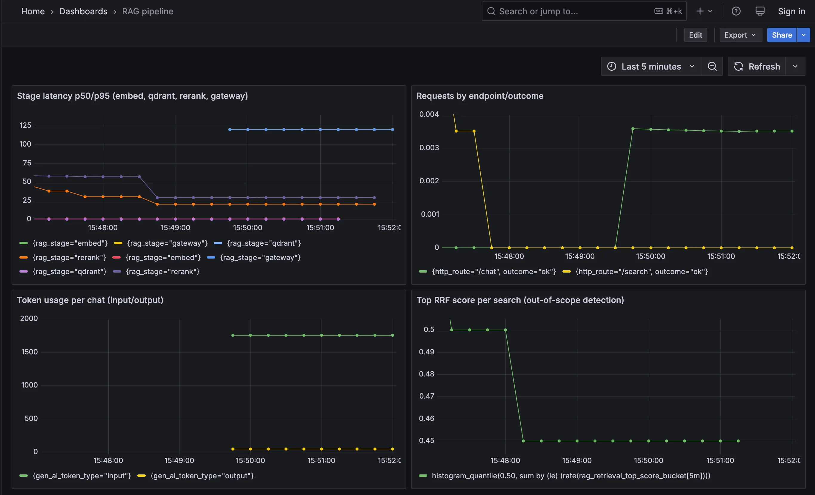
The retrieval service emits OpenTelemetry metrics following the GenAI semantic conventions, scraped by a self-hosted Prometheus and displayed in Grafana:

• gen_ai.client.operation.duration: latency per model call (embed, rerank, chat completion)
• rag.retrieval.stage.duration: latency per pipeline stage (embed, qdrant, rerank, gateway)
• gen_ai.client.token.usage: input and output tokens per chat
• rag.retrieval.top_score: distribution of top fusion scores, which separates in-scope from out-of-scope questions
• Request counters per endpoint and outcome

The dashboard makes the tuning levers visible: the rerank stage dominates the pre-LLM latency at 50 candidates, and the gateway stage shows the CPU tier's prompt processing speed. Both are knobs, not mysteries.

kubectl apply -f k8s/rag/observability/prometheus.yaml
kubectl apply -f k8s/rag/observability/grafana.yaml
kubectl -n rag port-forward svc/grafana 3000:3000
# open http://localhost:3000, dashboard "RAG pipeline"

k8s/rag/observability/prometheus.yaml
k8s/rag/observability/grafana.yaml

What broke along the way

Polished diagrams hide the fact that most of the design time went into failures. The honest list, because it is the part we would have wanted to read before starting:

• TEI would not start, at any memory limit. Its default backend (candle) was OOM-killed during model warmup at 2, 3, 4 and even 6 Gi. The fix was not more RAM but a different backend (ONNX Runtime), an explicit pooling mode (--pooling last-token, the ONNX export ships no pooling config), and a small --max-batch-tokens, because warmup memory scales with that value. A larger batch size also rejected bulk requests with HTTP 422 until --max-client-batch-size was raised.
• llama.cpp was bizarrely slow. It answered a 4-token embedding request in about 3.3 seconds, on an idle node, with or without CPU limits. We never fully explained that number, and we did not have to: TEI was six times faster, so the benchmark picked the winner and llama.cpp was deleted. Benchmarks exist precisely so you do not have to debug every mystery.
• The planned node size was wrong. The cost-optimized e2-standard-2 pool could not host either embedding server in any configuration we tried. The pool moved to e2-standard-4, about $50 per month more. The initial plan also assumed 2 Gi would be enough for an embedding server. It was not.
• My own latency budgets were fantasies. I had written "batch of 100 chunks in under 5 seconds" into the plan. A 0.6B model on shared e2 cores does about 180 tokens per second, so that batch takes minutes, not seconds. The query path budget (one short embedding under 100 ms) landed at about 110 ms and we accepted it. Budgets are hypotheses too; write them down, then let measurements correct them.
• Google Managed Prometheus silently exported nothing. Scraping worked, the configuration was correct, and still no metrics of any kind reached Cloud Monitoring, not even native GKE ones, even after fixing a real IAM gap on the node service account. Instead of sinking more time into a platform black box, we self-hosted a plain Prometheus in the namespace and had working dashboards the same hour. The GMP question stays open as a platform issue to revisit.

Global architecture

The rag namespace sits in front of the stack. Questions go through the retrieval API first, and only the final prompt (question plus retrieved context) reaches the Envoy gateway, which then serves it with the tiered models from the previous article.

The full deploy runbook lives in k8s/rag/README.md, and the deep technical reference in docs/rag-implementation.md.

Conclusion

Adding this RAG namespace aligns with the late 2025 and 2026 best practices: structure-aware chunking, hybrid search, cross-encoder reranking, and evaluation as a first-class metric. Quality of retrieval beats volume of datapoints, especially with a small corpus where every miss is visible.

The practices are still shifting, mostly toward agentic loops where a planner decides when and how to retrieve, and toward richer context per chunk. Those are sequenced, not skipped: the evaluation harness and the monitoring are already in place, so each of them will have to prove its value on the same golden set before earning a place in the stack.

Where to go next

If you want to reproduce this learning path or extend it, this is the order I would follow. Each step is small, has a clear trigger, and teaches a distinct skill:

1. Scale the corpus, then watch the eval break. Move a few hundred real documents into the bucket, extend the golden set in the same change, and re-measure. This is where you learn what chunking actually costs, because hit@5 will drop and the failure modes (tables split mid-way, ambiguous fragments, acronym collisions) finally become visible.
2. Contextual retrieval, now with a measurable goal. An LLM writes one context sentence per chunk at ingestion time (Anthropic reports 35 to 67 percent fewer failed retrievals). On my current corpus it had no headroom, so it was deferred. After step 1 it becomes a real experiment with a before and after report, and it teaches you ingestion-time LLM usage without touching the query path.
3. Agentic retrieval. Let a planner call the pipeline as a tool (the Qdrant MCP server is the natural entry) instead of forcing every question through retrieval. This is the 2026 pattern, and it forces a real design question I still owe an answer: how should it coexist with the semantic router, which already does a primitive form of triage?
4. Cost per query. The metrics already record tokens per chat and node hours are known. The remaining work is arithmetic: cost per 1,000 queries, self-hosted versus a managed RAG service. That article completes the trilogy: quality, latency, cost.
5. Answer-level evaluation. My harness measures retrieval, not answers. Ragas-style metrics (faithfulness, context precision) close that gap, and building them teaches you where hallucinations actually come from when retrieval is already correct.

The pattern behind all of them is the real lesson of this project: pick one change, measure it against a set you trust, keep it only if the numbers move. Everything else is decoration.